Backtesting a Pairs Trading Strategy
This is a revised version of the original Medium post. The trading period in this version was halved (from one quarter or 63 days to a half quarter or 31 days). The pairs trading results are significantly better.
This notebook performs a backtest on a pairs trading strategy based on pairs selection using correlation and cointegration. The backtest is designed to resemble the actual trading of the strategy. The Python code in this notebook would serve as a model for the Java code that would be used to trade the strategy (I would never deploy Python in an application that required high reliability).
Pairs trading is a strategy that dates to the 1980s.
Pair trading was pioneered by Gerry Bamberger and later led by Nunzio Tartaglia’s quantitative group at Morgan Stanley in the 1980s.
Pairs Trade in Wikipedia
The market-neutral nature of the pairs trading strategy makes it attractive since the strategy is less likely to experience significant drawdowns during market downturns.
There is a fairly sizable literature on pairs trading, consisting of academic articles, blog posts, and a few books. Many of these references suggest that the strategy can yield attractive returns with lower risk.
Unlike many of the references on pairs trading, this notebook was written to evaluate the strategy for actual trading. If the strategy proved to be attractive, I would have written Java code to trade this strategy. With the possibility of risking my money on this strategy, I have tried to be careful in the analysis. I compare the pairs strategy to an equivalent portfolio of randomly selected pairs to determine whether the statistical tests for mean reversion deliver increased returns over the random pairs.
A rolling six-month in-sample period is used to evaluate correlation and cointegration to select pairs. Following the in-sample period there is a trading period over which the pairs may be traded. The pairs trading results are sensitive to the number of days in the out-of-sample. The pairs trading results for a one quarter out-of-sample period are almost exactly the same as the results for the random pairs. When the trading period is reduced to half of a quarter (32 days), the pairs trading results are almost double the results from the random pairs.
The source for this notebook can be found on GitHub (https://github.com/IanLKaplan/pairs_trading/blob/master/pairs_trading_backtest.ipynb)
This notebook is a sequel to the notebook Exploratory Statistics of Pairs Trading (https://github.com/IanLKaplan/pairs_trading/blob/master/pairs_trading.ipynb). The previous notebook explores the algorithms for selecting pairs and the statistics of pairs trading. This statistical exploration provides the foundation for the strategy that is backtested in this notebook. For a discussion of pairs trading, the algorithms used to select pairs, and the background for the strategy that is backtested in this notebook, please see the previous notebook.
Pairs Trading Strategy
Shorting Stocks in Pairs Trading
Pairs trading is a market-neutral long/short strategy where the long and short positions for a pair have approximately equal dollar values when the position is opened. A profit is realized when there is mean reversion in the spread between the prices of a pair.
This section discusses the mechanics of taking a short position in a stock. A short position in a stock is a margin loan and is more complicated than a long position.
When a stock is “shorted”, the stock is borrowed and then immediately sold, realizing cash. For example, if 100 shares at a current market price of 10 are shorted, the brokerage account will be credited with 1000 (100 x 10). At some point in the future, the borrowed stock must be paid back by buying the stock at the current market price. A short position is profitable when the market price of the stock goes down. For example, if the market price of the stock is shorted at 10 and goes down to 6, there is a profit of 4 per share (4 x 100 = 400).
Short positions can have an unlimited loss when the stock price goes up. For example, if the market price of the 10 stock rises to 14 per share, there is a 400 loss on the 100-share purchase. If the stock price doubles to 20 there will be a loss of 10 per share or 1000 for the short position.
Shorting stocks is often considered a risky investment strategy because of the potential for unlimited loss. Pairs trading is a market-neutral strategy where there is a long position that is approximately equal in dollar value to the short position. The pairs that are traded are chosen from the same industry sector and are highly correlated and cointegrated. If the market price of the shorted stock rises, the value of the long member of the pair should rise as well. The profit in the long position will tend to offset the loss in the short position. This makes the pairs trading strategy less risky than a short-only strategy.
When a stock is shorted, the stock is borrowed from the broker. This is treated as a margin loan. The brokerage requires that the customer maintain a balance with liquid assets of 150 percent of the amount borrowed. This includes the proceeds of the short sale, plus 50 percent. For example, if 100 shares of a 10-dollar stock are shorted, the account will be credited with 1000. The account must also have an additional balance of 500. The margin requirement can be met with cash or highly tradable “blue chip” stocks (e.g., S&P 500 stocks).
The pairs trading strategy is cash efficient. For example, a long position of 1000 and a short position of 1000 can be opened with only 500 in cash or highly tradable assets.
When the pair spread crosses a threshold, a long-short position is opened in the pair. This threshold is the mean plus or minus some delta amount. The dollar value of the long and short positions will be approximately equal (they will usually not be exactly equal because we are trading whole share amounts). When the spread value crosses the threshold:
- Open the short position. This will result in cash from the short sale.
- The proceeds from the short sale are used to pay for the long position. An additional amount of cash may be needed for the long position.
This is summarized in the equations below. The “/” operator is an integer divide operator:

If the cost of the long position is greater than the cash realized from the short position, additional cash will be allocated for the long position.
Example:
If our trading capital is 100,000 we can open a 200,000 long and 200,000 short position, given a 50 percent margin. Ideally the margin funds could be allocated to an asset like a bond ETF which pays a monthly dividend.
If we trade 100 pairs, then each pair is allocated 1,600 for the long and short positions.
Stock A (the long position) is 63 per share and stock B (the short position) is 54 a share. We open the short position first to obtain the cash for the long position. The division operations are integer divisions.

Interactive Brokers charges a yearly fee for short positions is 0.25 percent or 0.25/360 percent per day that the position is held. This is small enough that the short-interest cost can be ignored.
The pairs trading strategy will have a portfolio of short and long positions which are opened and closed as the pair spread moves. At any time, the aggregate value of the short positions and the long positions, plus margin cash, must be within the margin requirements. If there is a liquidity deficit relative to the margin, IB will liquidate the deficit amount times 4 (ouch!)
When the short position is opened there must be a margin of at least 50 percent. Interactive brokers marks to market in real-time. The SEC regulation T requires that there be a margin of at least 25% for open short positions.
Interactive Brokers Margin reference
Stock Price Data Issues
The backtest in this notebook uses the daily close price for the stocks. If a large number of stocks are traded (i.e., 100 stocks) a Java trading application would use the intraday prices. The intraday prices will generally not be the same as the close price. The purpose of the backtest in this notebook is to provide an indication of the profitability and risk of the pairs trading strategy, so this difference is acceptable.
In-sample and out-of-sample time periods
The pairs trading set is constructed by looking back over the past in-sample period. The out-of-sample period is the trading period.
- In-sample period: six months (126 trading days)
- Out-of-sample (trading) period: three months (31 trading days). A 31-day period should be long enough to capture mean reversion while still maintaining the statistical characteristics of the in-sample period. By using a relatively short out-of-sample period risk of holding pairs is reduced and the statistics for pairs selection can be calculated after the out-of-sample period.
Data Snooping
Data snooping takes place when the performance of a strategy is observed and used to adjust strategy parameters. Future information that would not have been available over the strategy back-test can result in differences between strategy backtest results and actual trading results.
The length of the out-of-sample trading period was adjusted from one quarter to a half quarter on the basis of observed pairs trading results. The theoretical justification for this is that a shorter out-of-sample period is more likely to statistically resemble the in-sample period used for pairs selection.
Observations of the pairs performance was also used to remove the limitation that pairs have unique stocks.
The adjustments to the strategy are broad and data snooping is not obviously an issue in these cases.
Strategy
Get pairs for each S&P 500 industrial sectors
For each 126 day in-sample window (moving forward every 63-days):
- Select the pairs with close price series correlation greater than or equal to 0.75
- Select the high correlation pairs that show Granger cointegration
- Sort the pair spread time series by volatility (high to low volatility). Higher volatility (standard deviation) pairs are more likely to be profitable.
- Select the top N pairs from the sorted pair list
Out-of-sample trading period
The pairs trading backtest is intended to be as close to actual trading as possible in order to understand whether this strategy is worth pursuing for actual trading.
At the start date of the backtest, the total cash available is N dollars (e.g., 100,000). With a required margin of 50 percent, this would allow us to have a position of 2N for the long and short positions (e.g., for 100,000 cash, long and short positions of 200,000 each).
Positions are opened for whole share values.
At the end of each out-of-sample trading period, any open positions will closed.
For each pair (in the N pair set) in the out-of-sample trading period:

Filtering Pairs
From the universe of S&P 500 industry sector stock pairs, pairs are first selected for high correlation and then for cointegration using the Engle-Granger test (linear regression and the ADF test).
The distribution of the standard deviation of the pairs spread is shown below.

Unstable Statistics
In the pairs trading literature, a central concept is that the statistics that are calculated for the in-sample period are stable (stationary) and will persist in the out-of-sample trading period. The previous notebook, Exploratory Statistics of Pairs Trading, looks at the stability of correlation and cointegration between adjacent periods. As it turns out, high correlation is consistent between adjacent periods only about 50 percent of the time. Cointegration is persistent between adjacent periods even less, only about 40 percent of the time.
Pairs trading assumes that the spread time series is “stationary”, and that it has a constant mean and standard deviation. Unfortunately, this is not necessarily true, even for spread time series that are mean reverting in the in-sample and out-of-sample period.
The plots below show the normalized time series for a pair and the spread time series. The plots show the mean as a thick horizontal line. The in-sample mean is near zero. The out-of-sample mean is far from zero. In both of the plots of the spread time series, the in-sample deviation is shown in the dotted line. As it turns out, the out-of-sample standard deviation is around twice the in-sample standard deviation.


Bollinger Band
The pairs trading algorithm opens pairs positions when the spread is above or below the mean by some amount. In the pairs trading literature, the spread is a stationary time series, with a mean that is relatively constant between the in-sample and out-of-sample time periods. As the above example shows, in practice, the mean is often not constant between the in-sample and out-of-sample periods.
The mean is constantly changing, so a rolling mean is calculated on a look-back window. A rolling standard deviation is also calculated on the same lookback window. When the spread is above or below the rolling mean by some amount, a pairs position is opened. When there is an open pair position and the spread crosses the rolling mean, the position is closed.
This is a Bollinger Band. In the pairs trading literature, a number of articles use Bollinger Bands for pairs trading. See Pairs Trading in Practice by Jonathan Kinlay, Feb 18, 2019.
The common Bollinger band limit is two standard deviations. This seems to work well for pairs trading. I have tried both one and two standard deviation bands. The two standard deviation band results in higher portfolio profits and less trading.
The plots below show the spreads for the in-sample and out-of-sample pairs, along with Bolinger Bands using the running mean and standard deviation.


Number of Pairs
Cointegration between pairs is persistent between the in-sample and out-of-sample periods in only 40 percent of the pairs. In order to capture the cases where cointegration is persistent, there must be a sufficient number of pairs. Risk is also limited by limiting the cash allocated for any single pairs position.
In this backtest 100 pairs are used. The pairs are selected from industry sectors, as described above. If the stocks in the pairs were unique, so that pairs do not share the same stock, there would be 200 unique stocks. This is would be almost half of the S&P 500 stock set. A pairs trading strategy that uses such a stock set runs the risk of reproducing the performance of the S&P 500 (the objective of the pairs trading strategy is to beat the S&P 500 in either return or risk or both).
Removing the requirement that the selected cointegrated pairs must have unique stocks results in better pairs trading performance and is less likely to mirror the S&P 500. The increased performance comes with the risk of concentration in stocks, since a stock may exist in multiple pairs.
The histogram below shows the distribution of stocks within all of the pairs chosen in the backtest period. Around half of the pairs have unique stocks. In about a quarter of the pairs, stocks are shared by two pairs. The remaining quarter has pairs with stocks shared by three or more pairs. This plot suggests that concentration in a set of stocks is not an issue.

Opening Pairs Positions and Margin
When the spread moves away from the running mean by 2σ a pair position is opened with long and short positions of approximately equal dollar value (we are buying whole shares, so it may not be possible to have exactly equivalent positions).
There are 100 pairs, so 1/100 of the capital is allocated for the pair. If we have 100,000 in trading capital, 1,000 is allocated for each pair. This supports a 2,000 short position and a 2,000 long position. The long position is used to partially meet the margin requirement for the short position. When a short position is opened there must be 50% in liquid assets or cash for the margin (this is required by the US SEC Regulation T). In this case, we have 1,000 for the 50% margin. When the short is opened, the stock is borrowed and immediately sold. The proceeds of the short sale are used to open an equivalent 2,000-long position. The result is a relatively market-neutral position with 2,000-short and 2,000 long in the stock pair.
Once the position is opened, the prices for the stocks in the pair move. As the prices move, Regulation T requires a margin of at least 25% for the short positions, in addition to a long position that balances 100% of the short position. In the worst case, if the short position goes up and the long position goes down, additional margin could be required.
The pairs trading backtest estimates the required margin for open pairs positions. In the backtest, which is using close prices instead of intraday prices, the margin requirement never crosses the margin reserve composed of the long position plus the margin cash (or other securities).
When a pairs trade results in a profit, this profit is added to the initial trading capital and is used to open future positions.

The plot above shows the required margin in excess of the long position in a pair. The current cash balance is also shown. This starts out with the initial investment and grows as the pairs trading strategy yields profits.
Distributions
One way to check the reliability of backtest results is to look at the return statistics.
When a pairs trade is closed there will be a return for both the short and the long pairs positions. These pair positions make up a two-asset portfolio where each asset (the long and short positions) are approximately 50 percent of the portfolio. Multiple pairs may be closed on a single day. This forms a portfolio for the day. The returns for each pair can be added together as a weighted sum, where the weight is 1/num_pairs, where num_pairs is the number of pairs that are closed on that day.
The return distribution is plotted below. The return distribution looks like the return distributions that can be expected for stock market assets.

When the pair is closed there will be a profit or loss. Calculating the portfolio value by adding the profit or loss for a day is a simpler calculation than the return calculation. The amount of cash (or loss) is per day plotted below.
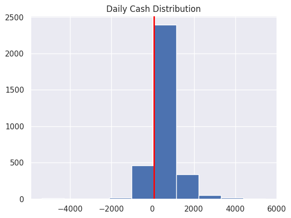
The previous statistics are from the daily trade information. The portfolio return can also be calculated from the running portfolio value. This distribution is shown below. This distribution does not match the return distribution.

Open Pairs Positions
A long/short pair position is opened when the pair spread is 2σ above or below the running mean. When the spread crosses the mean, the pairs position is closed. The plot below shows the number of days a pairs position is open.

The plot below shows the distribution of the number of open pair positions per day. New pairs positions are not opened within 15 days of the end of the quarter, since they would be unlike to be open long enough to mean revert and close.

At the start of the out-of-sample trading period, a new set of pairs is chosen using the past in-sample period. Pairs are opened and closed as we move forward in time. Not all pairs positions will mean revert and close by the end of the quarter. Any open pairs positions are closed at the end of the trading period.
total profit (loss): 236994.0 min val: -35870.0 max val: 12421.0
total percent positive trades: 58.83Pairs Portfolio vs a Random Portfolio
A portfolio of 100 random pairs is compared to the portfolio of pairs selected using correlation and cointegration. The random pairs are created by selecting stocks from the industry sector stock universe. The random pairs are traded in the same way that the cointegrated pairs are traded (e.g., the spread is calculated and trades are opened with the spread moves sufficiently away from the mean and closed with it return to the mean).
By comparing the performance of pairs selected for mean reversion with random pairs we can get some measure of whether the statistical tests yield better porfolio performance.

This plot suggests that the application of correlation and cointegration delivers better returns than a randomly selected set of pairs.
Pairs Trading vs SPY: Five Years and One Year
The plots below show the performance of the pairs trading strategy in the last five years and the last year.
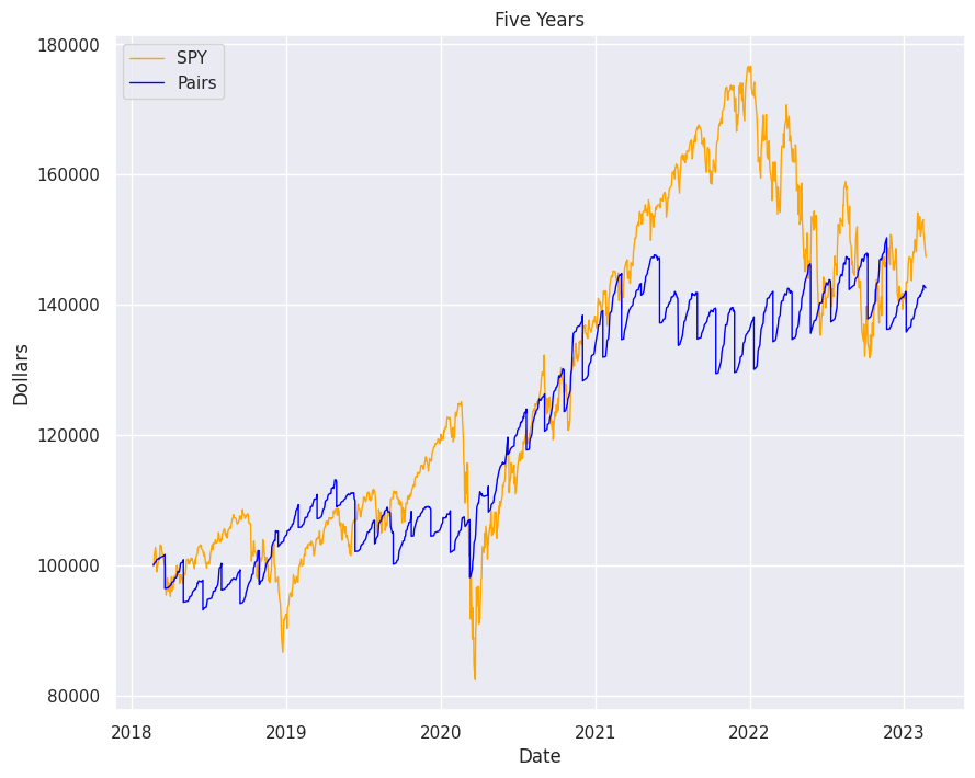

The trading period for the strategy is half of a quarter (31 trading days). Before the start of the trading period, the next set of pairs is selected using correlation and cointegration over a look-back period of 126 trading days (six months). Pairs trades are opened at the start of the quarter as the pair spread sufficiently diverges from the mean. The pairs position is closed when the spread returns to the mean. All open pairs positions are closed at the end of the quarter.
As the one-year plot shows, profits increase through the quarter. There is a drawdown at the end of the trading period when any open pairs positions are closed. Presumably, the drawdown is a result of pairs that drifted together, resulting in a net loss when the pair is closed.
No new pairs positions are opened within 10 days of the end of the trading period (see the day_limit variable in the HistoricalBacktest class). This limit was chosen because, in most cases, there would not be sufficient time for a pair to mean revert.
There may be additional algorithmic techniques to limit the losses in the unprofitable pairs. For example, if the pairs position crosses a loss threshold, it might be closed to limit the loss.
Discussion
Returns for Cointegrated and Random Pairs

The yearly returns (as a percentage) for the pairs portfolio, the random pairs portfolio, and SPY are shown above. The yearly returns for the cointegrated pairs are almost double the returns for the random pairs. The random pairs use a seeded random number generator, so the random pairs selected will always be the same over multiple runs of the notebook.
These results suggest that a pairs trading strategy that uses correlation and cointegration to select pairs delivers returns that are, on average, higher than a strategy that uses pairs constructed from randomly selected stocks. The pairs strategy also has low yearly drawdown. The worst performance, in 2012, was a loss of a little less than two percent.
The length of the trading period has a significant impact on the pairs trading results. For a one-quarter out-of-sample trading period, correlation and cointegration are no better at selecting pairs that will mean revert than randomly selected pairs. The shorter half-quarter trading period delivers returns that are almost double the returns of the random pairs.
There are many articles on the pairs trading strategy and it is covered in books like Algorithmic Trading by E.P. Chan and Pairs Trading by Ganapathy Vidyamurthy. Although the articles and books cover the in-sample calculations for cointegration, very few examine the persistence of this statistic. Very few references use backtests that closely resemble the actual trading of the strategy.
Correlation and cointegration seem to have a rapid decay between the in-sample and the out-of-sample trading period (see Exploratory Statistics of Pairs Trading).
The pairs trading strategy is a market-neutral strategy and has a significantly lower maximum drawdown than the S&P 500. The pairs strategy is trading lower drawdowns for performance that lags the S&P 500 in some years.
Disclaimer
This notebook is not financial advice, investment advice, or tax advice. The information in this notebook is for informational and recreational purposes only. The investment products discussed (ETFs, mutual funds, etc.) are for illustrative purposes only. This is not a recommendation to buy, sell, or otherwise transact in any of the products mentioned. Do your own due diligence. Past performance does not guarantee future returns.