Exploratory Statistics of Pairs Trading

by Ian Kaplan

This Jupyter notebook explores pairs trading strategies. This document is available from the GitHub repository https://github.com/IanLKaplan/pairs_trading

Pairs trading is an approach that takes advantage of the mispricing between two (or more) co-moving assets, by taking a long position in one (many) and shorting the other(s), betting that the relationship will hold and that prices will converge back to an equilibrium level.

Definitive Guide to Pairs Trading available from Hudson and Thames

Pairs trading is sometimes referred to as a statistical arbitrage trading strategy.

Statistical arbitrage and pairs trading tries to solve this problem using price relativity. If two assets share the same characteristics and risk exposures, then we can assume that their behavior would be similar as well. This has the benefit of not having to estimate the intrinsic value of an asset but rather just if it is under or overvalued relative to a peer(s). We only have to focus on the relationship between the two, and if the spread happens to widen, it could be that one of the securities is overpriced, the other is underpriced, or the mispricing is a combination of both.

Definitive Guide to Pairs Trading available from Hudson and Thames

Pairs trading algorithms have been reported to yield portfolios with Sharpe ratios in excess of 1.0 and returns of 10% or higher. Pairs trading takes both long and short positions, so the portfolio tends to be market neutral. A pairs trading portfolio can have drawdowns, but the drawdowns should be less than a benchmark like the S&P 500 because of the market-neutral nature of the portfolio. The lower, market-neutral, structure of a pairs trading portfolio means that the portfolio will have a lower return than a comparable benchmark like the S&P 500.

Markets tend toward efficiency and many quantitative approaches fade over time as they are adopted by hedge funds. Pairs trading goes back to the mid-1980s. Surprisingly, pairs trading still seems to be profitable. One reason for this could be that there are a vast number of possible pairs and a pairs portfolio is a faction of the pairs universe. This could leave unexploited pairs in the market. Pairs trading may also be difficult to scale to a level that would be attractive to institutional traders, like hedge funds, so the strategy has not been arbitraged out of the market.

Mathematical finance often uses models that are based on normal distributions, constant means, and standard deviations. Actual market data is often not normally distributed and changes constantly. The statistics used to select stocks for pairs trading assume that the pair distribution has a constant mean and standard deviation (e.g., the pairs spread is a stationary time series). As this notebook shows, this assumption is statistically valid about forty percent of the time.

Overview

This notebook and the associated GitHub repository explore the statistics of pairs trading.

The primary references used for this notebook are the books Pairs Trading by Ganapathy Vidyamurthy and Algorithmic Trading by Ernest P. Chan. Several articles and web references were valuable in understanding the pairs selection algorithms.

A pairs trading strategy attempts to find a pair of stocks where the weighted spread between the stock prices is mean reverting.

Implementing the pairs trading strategy involves two logical steps:

1. Pairs selection: Identify a pair of stocks that are likely to have mean-reverting behavior using a lookback period.
2. Trading the stocks using the long/short strategy over the trading period. This involves building a trading signal from the weighted spread formed from the close prices of the stock pair. When the trading signal is above or below the mean by some threshold value, a long and short position is taken in the two stocks.

Pairs Selection

S&P 500 Industry Sectors

In this notebook, pairs are selected from the S&P 500 stock universe. These stocks have a high trading volume, with a small bid-ask spread. S&P 500 stocks are also easier to short, with lower borrowing fees and a lower chance that a short position will be called back.

In pairs selection, we are trying to find pairs that are cointegrated, where the price spread has mean-reverting behavior. Just as there can be spurious correlation there can be spurious cointegration, so the stock pair should have some logical connection. In the book Pairs Trading (Vidyamurthy) the author discusses using factor models to select pairs with similar factor characteristics.

Factor models are often built using company fundamental factors like earnings, corporate debt, and cash flow. In many cases, the company factors that affect S&P 500 companies are broad economic factors that are not obviously useful in choosing pairs for mean reversion trading. Companies in completely different industry sectors may have similar fundamental factors. When selecting pairs we would like to select stocks that are affected by similar market forces. For example, energy sector stocks tend to be affected by the same economic and market forces.

In lieu of specific factors, the S&P 500 industry sector is used as the set from which pairs are drawn. Although not perfect, the industry sector will tend to select stocks with similar behavior, while reducing the universe of stocks from which pairs are selected.

Reducing the universe of stock pairs is important because, even with modern computing power, it would be difficult to test all possible stock pairs in the S&P 500, since the number of pairs grows exponentially with N, the number of stocks.

The S&P 500 component stocks (in 2022) and their related industries have been downloaded from barchart.com. The files are included in the GitHub repository.

The S&P 500 industry sectors are:

1. Consumer discretionary
2. Consumer staples
3. Energy
4. Financials
5. Health care
6. Industrials
7. Infotech
8. Materials
9. Real estate
10. Communication services
11. Utilities

The stocks from the Barchart list include stocks for the same company, with different classes (e.g., class A, class B, or class C stocks). The list of stocks is filtered to remove all but the lowest stock class (e.g., if there is a class B stock, the class A stock is removed from the list).

Stock Market Close Data

The data used to model pairs trading in this notebook uses close price data for all of the S&P 500 stocks from the start date to yesterday (e.g., one day in the past).

In other models (see Stock Market Cash Trigger and ETF Rotation) the close price data was downloaded the first time the notebook was run and stored in temporary files. The first notebook run incurred the initial overhead of downloading the data, but subsequent runs could read the data from local temporary files.

For the S&P 500 stock universe, downloading all of the close price data the first time the notebook is run would have an unacceptable overhead. To avoid this, the data is downloaded once and stored in local files. When the notebook is run at later times, only the data between the end of the last date in the file and the current end date will be downloaded.

There are stocks in the S&P 500 list that were listed on the stock exchange later than the start date. These stocks are filtered out, so the final stock set does not include all of the S&P 500 stocks.

Filtering stocks in this way can create a survivorship bias. This should not be a problem for back-testing pairs trading algorithms through the historical time period. The purpose of this backtest is to understand the pairs trading behavior. The results do not depend on the stock universe, only on the pairs selected.

The table below shows the number of unique pairs for each S&P 500 sector and the total number of pairs. By drawing pairs from sectors, rather than the whole S&P 500 set of stocks, the number of possible pairs is reduced from 124,750.

╒════════════════════════╤══════════════╤═════════════╕
│                        │   num stocks │   num pairs │
╞════════════════════════╪══════════════╪═════════════╡
│ materials              │           22 │         231 │
├────────────────────────┼──────────────┼─────────────┤
│ information-technology │           54 │        1431 │
├────────────────────────┼──────────────┼─────────────┤
│ consumer-discretionary │           47 │        1081 │
├────────────────────────┼──────────────┼─────────────┤
│ health-care            │           52 │        1326 │
├────────────────────────┼──────────────┼─────────────┤
│ communication-services │           16 │         120 │
├────────────────────────┼──────────────┼─────────────┤
│ energies               │           16 │         120 │
├────────────────────────┼──────────────┼─────────────┤
│ consumer-staples       │           28 │         378 │
├────────────────────────┼──────────────┼─────────────┤
│ utilities              │           24 │         276 │
├────────────────────────┼──────────────┼─────────────┤
│ industrials            │           58 │        1653 │
├────────────────────────┼──────────────┼─────────────┤
│ financials             │           58 │        1653 │
├────────────────────────┼──────────────┼─────────────┤
│ real-estate            │           28 │         378 │
├────────────────────────┼──────────────┼─────────────┤
│ Sum                    │          403 │        8647 │
╘════════════════════════╧══════════════╧═════════════╛

Lookback Time Period

Pairs are selected for trading using a lookback period. The longer the lookback period, the less error there will be in the selection statistics, assuming that the data is stable (e.g., constant mean and standard deviation). Stock price time series are not stable over time, however. The mean and the standard deviation change, as do other statistics like correlation and cointegration (mean reversion).

In using a lookback period to choose trading pairs we are making the assumption that the past will resemble the future trading period (as we shall see, this is not true in the majority of cases). The longer the lookback period, the less likely it is that the statistics will match the trading period. This creates a tension between statistical accuracy and statistics that are more likely to reflect the future trading period.

A half-year period is used for the lookback period. In practice, the statistics for a year period (252 trading days) and a six-month period (126 trading days) seem to be similar. We assume that the six-month period will more accurately resemble the future trading period.

Mean Reversion

A single stock price series is rarely stationary and mean reverting. In pairs trading, we are looking for stock pairs where the stock price spread time series is stationary and mean in the in-sample (lookback) period. We are making a bet that the spread time series will also be stationary and mean reverting in the out-of-sample trading period.

When a pair forms a mean-reverting, stationary time series, it is referred to as a cointegrated time series.

This (linear) price data combination of n different time series into one price data series is called cointegration and the resulting price series w.r.t. financial data is called a cointegrated pair.

Cointegration Analysis of Financial Time Series Data by Johannes Steffen, Pascal Held and Rudolf Kruse, 2014

https://www.inf.ovgu.de/inf_media/downloads/forschung/technical_reports_und_preprints/2014/02_2014.pdf

In the equations below, s is a stationary mean reverting weighted spread time series, PA is the price series for stock A, PB is the price series for stock B and β is the weight factor (for one share of stock A there will be β shares of stock B).

When s is above the mean at some level, delta (perhaps one standard deviation), a short position will be taken in stock A and a long position will be taken in β shares of stock B. When s is below the mean at some level (perhaps one standard deviation) a long position will be taken in stock A and a short position will be taken in β shares of stock B.

In identifying a pair for pairs trading, a determination is made on whether s is mean reverting. The process of determining mean reversion will also provide the value of β.

Testing for Cointegration and Mean Reversion

Highly correlated pairs are selected from a common industry sector. Once a pair with high correlation is identified, the next step is to test whether the pair is cointegrated and mean reverting. Two tests are commonly used to test for mean reversion:

1. Engle-Granger Test: Linear Regression and the Augmented Dickey-Fuller (ADF) test
2. The Johansen Test

Each of these tests has advantages and disadvantages, which will be discussed below.

Engle-Granger Test: Linear Regression and the Augmented Dickey-Fuller Test

Two linear regressions are performed on the price series of the stock pair. The residuals of the regression with the highest slope are tested with the Augmented Dickey-Fuller (ADF) test to determine whether mean reversion is likely.

Linear regression is designed to provide a measure of the effect of a dependent variable (on the x-axis) on the independent variable (on the y-axis). An example might be body mass index (a measure of body fat) on the x-axis and blood cholesterol on the y-axis.

In selecting pairs, we pick pairs with a high correlation from the same industry sector. This means that some process may be acting on both stocks. However, the movement of one stock does not necessarily cause movement in the other stock. Also, both stock price series are driven by an underlying random process. This means that linear regression is not perfectly suited for analyzing pairs. Two linear regressions are performed since we don’t know which stock to pick as the dependent variable. The regression with the highest slope is used to analyze mean reversion and build the cointegrated time series.

The slope in the linear regression performed for the (Engle) Granger test is the weight value for the equation above. A linear regression intercept is also available, along with the confidence level of the cointegration process (e.g., 90%, 95%, and 99% confidence).

Example: AAPL/MPWR/YUM

AAPL (Apple Inc) and MPWR (Monolithic Power Systems, Inc) are in the technology industry sector. YUM (Yum brands) is a food company in a different industry sector. The correlations of MPWR and YUM with AAPL in the first half of 2007 are shown below. AAPL and MPWR are both technology sector stocks, while YUM brands is a food company. Other than overall stock market dynamics, we would not expect AAPL and YUM to be correlated, so this appears to be an example of a false correlation.

╒══════╤════════╤═══════╕
│      │   MPWR │   YUM │
╞══════╪════════╪═══════╡
│ 2007 │   0.91 │  0.88 │
╘══════╧════════╧═══════╛

Monolithic Power Systems, Inc. (MPWR) stock grew at a rate that was similar to Apple’s, although the overall market capitalization is a faction of Apple’s now. I was unfamiliar with MPWR until I wrote this notebook. Bloomberg describes MPWR’s business as:

Monolithic Power Systems, Inc. designs and manufactures power management solutions. The Company provides power conversion, LED lighting, load switches, cigarette lighter adapters, chargers, position sensors, analog input, and other electrical components. Monolithic Power Systems serves customers globally.

A brief digression: Apple is now (2022) one of the most valuable companies in the world. A number of investment funds bought Apple shares and were able to beat the overall market for the years when Apple had exceptional growth.

My father invested in such a fund. Every quarter they sent out a “market outlook” newsletter. This newsletter was filled with blather to make fund investors think that the people managing the fund had special insight into the stock market (which justified the fees the fund charged). In fact, their only insight was their position in Apple stock. When Apple’s share price plateaued, so did the fund's returns.

Pairs may have a high correlation without being cointegrated. The (Engle) Granger test shows that in the first half of 2007 AAPL and MPWR were cointegrated at the 99% level.

Granger test for cointegration (AAPL/MPWR): 
cointegrated: True, confidence: 1, weight: 3.7, intercept: 1.05 (MPWR, AAPL)

The confidence level represents the error percentage. So 1 = 1% error or 99% confidence, 5 = 5% or 95% confidence, and 10 = 10% or 90% confidence.

The plot below shows the stationary spread time series formed by

The dotted lines are a plus one and minus one standard deviation. The intercept adjusts the time series so that the mean is zero.

AAPL and MPWR are both technology stocks that have some overlapping businesses (MPWR’s products are used by companies like Apple). We would expect that the two stocks might be cointegrated.

The test for cointegration is performed in a lookback period. The next period is the trading period where the close prices of the pair are combined with the weight (and perhaps the intercept) to form what we hope will be a stationary mean reverting time series that can be profitably traded.

The test below applies the Granger test to the second half of 2007 to see if mean reversion persisted. As the test results shows, this is not the case.

Granger test for cointegration (AAPL/MPWR): 
second half of 2007 cointegrated: False, confidence: 0, weight: 1.09, intercept: 14.56 (MPWR, AAPL)

The pair AAPL and YUM (Yum Brands, a food company) would not be expected to be cointegrated (although they have a surprisingly high correlation). As expected, the Granger test does not show cointegration and mean reversion.

Granger test for cointegration (AAPL/YUM): 
cointegrated: False, confidence: 0, weight: 2.45, intercept: 13.6 (YUM, AAPL)

Correlation and Cointegration

In choosing pairs for pairs trading, we are looking for a stock pair that is influenced by similar factors. The industry sector and high correlation can be used as the first filter for pairs.

The tests for cointegration may find that a stock pair with a low correlation value that is cointegrated and mean reverting. One example is AAPL and the technology sector stock GPN (Global Payments Inc.) For the first half of 2007, AAPL and GPN have a low correlation.

╒══════╤════════════════════════╕
│      │   Correlation AAPL/GPN │
╞══════╪════════════════════════╡
│ 2007 │                   0.32 │
╘══════╧════════════════════════╛

The normalized close prices for the two stocks in the first half of 2007 are shown below.

The Granger test shows that AAPL and GPN are cointegrated with 99% confidence (1% error). The Johansen test (see below) also shows that AAPL and GPN are cointegrated with 99% confidence.

Granger test for cointegration (AAPL/GPN)  : 
cointegrated: True, confidence: 1, weight: 0.56, intercept: 17.52 (GPN, AAPL)

The plot below shows the stationary time series formed from AAPL and GPN close prices.

Given their low correlation and unrelated businesses (computer and media hardware vs payments) this may be an example of spurious cointegration. If the cointegration is spurious, cointegration may be more likely to break down in a future time period and the pair may not be profitable to trade.

The Granger test for the second half of 2007 (e.g., the six months following the period above) is shown below:

Granger test for cointegration (AAPL/GPN): 
second half of 2007 cointegrated: False, confidence: 0, weight: 1.68, intercept: 11.46 (GPN, AAPL)

The Granger test shows that there is no cointegration in the six-month period following the first half of 2007, which reinforces the idea that the previous cointegration was spurious.

The Johansen Test

The Granger linear regression-based test can only be used for two assets. The Johansen test can be used on more than two assets.

The Johansen test uses eigenvalue decomposition for the estimation of cointegration. In contrast to the Granger test which has two steps: linear regression and the ADF test, the Johansen test is a single-step test that also provides the weight factors. There is no linear constant (regression intercept) as there is with the Granger test, so the Johansen result may not have a mean of zero.

The Johansen test and the Granger test do not always agree. The Johansen test is applied to AAPL/MPWR for the close prices from the first half of 2007. The Johansen test shows no cointegration, although the Granger test showed cointegration at the 99% confidence level.

Johansen test for cointegration (AAPL/MPWR), first half of 2007 : 
cointegrated: False, confidence: 0, weight: 3.71, (AAPL, MPWR)

In the research papers on cointegration, there doesn’t seem to be a consensus on whether the Granger or Johansen tests are better. Some authors suggest using both tests, but they don’t provide any empirical insight into why this might be advantageous.

Correlation

After selecting stocks based on their industry sector, the next filter used is the pair correlation of the prices.

Stocks that are strongly correlated are more likely to also exhibit mean reversion since they have similar market behavior. This section examines the correlation statistics for the S&P 500 sector pairs.

The lookback period for pairs selection is six months (126 trading days). As a first step, all of the S&P 500 sector pairs will be tested for correlation over the lookback period.

The windowed correlation is not stable. The plot below shows the correlation between two stocks, AAPL and MPWR, over windowed periods from the start date.

Since correlation is not stable, a stock pair that is highly correlated in one time period may be uncorrelated (or negatively correlated) in the next time period.

The histogram below shows the aggregate distribution of the pair correlation over all half-year time periods.

The pairs are selected from a common S&P industry sector, so there are a significant number of pairs that have a correlation above 0.75.

The plot below shows the number of pairs, in a half-year time period, with a correlation above a particular cutoff.

In the plot above, about 75% of the pairs are highly correlated around 2008. This corresponds to the 2008–2009 stock market crash caused by the financial crisis. The high correlation around the crash lends validity to the financial market maxim that in a market crash, all assets become correlated.

To the extent that correlation is a predictor for mean reversion, this also suggests that mean reversion statistics are volatile.

Correlation Statistics

This section looks at correlation statistics and their relation to cointegration:

• Stability of pairs correlation. When there is high pairs correlation (correlation greater than or equal to 0.75) in the past six months, how often is there a correlation in the next time period (correlation >= 0.60)?
• Is pairs correlation related to cointegration? For example, is a high correlation related to cointegration?

Stability of Correlation

For pairs trading to be a profitable strategy the statistics that are observed over a past period must persist into the next time period often enough to be profitable. For a pair that forms a stationary mean reverting spread time series in a past period, profitable pairs trading relies on this statistic holding over the out-of-sample trading period often enough to be profitable.

In this section, I look at whether a strong correlation between pairs makes it likely that there will be a strong correlation in the next time period. This is an important statistic for pairs trading because correlation is related to cointegration. If correlation persists between periods then cointegration and mean reversion might be more likely to persist. If correlation does not persist between time periods then cointegration may not be persistent.

The table below shows the dependence between the correlation in the past period and the correlation in the next period. The correlation in the past period is at least 0.75. The correlation in the next period is at least 0.60.

As the table above shows, about half (~49%) of the pairs with a high correlation are also highly correlated in the next time period.

Correlation and Cointegration

The histograms below show the relationship between correlation and cointegration, in the same half-year, in-sample period.

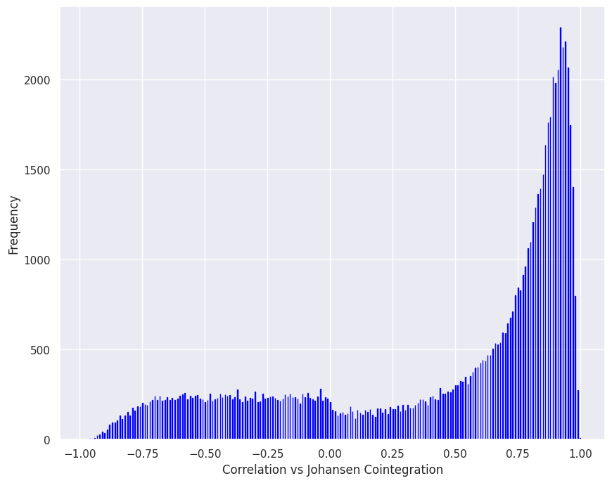
The histogram plots above show that there is a strong relationship between correlation and cointegration. That is, highly correlated pairs are more likely to be cointegrated.

The histogram below shows the relationship between correlation and cointegration where cointegration meets both the Granger and Johansen tests (e.g., Granger AND Johansen cointegration).

The histograms above show that correlation is an effective first filter for cointegration.

The histogram below shows the number of pairs that are highly correlated with Granger cointegration for each in-sample time period.

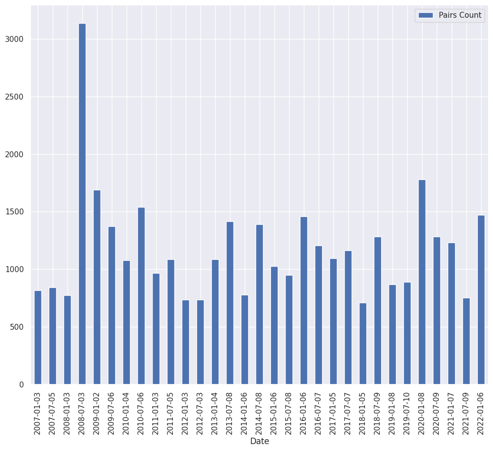
As we have seen, correlation increases in market crashes. The histogram above suggests that cointegration increases as well.

Stability of Cointegration

Cointegration for a pair is calculated over an in-sample look-back period. When a pair is found to be cointegrated, trading takes place in the out-of-sample period. For example, cointegration is calculated over a half-year look-back period. Trading, using the cointegration spread, might take place over a three-month out-of-sample period following the look-back period.

For a cointegrated pair, the spread time series is a stationary time series with a constant mean and standard deviation. The spread time series is mean reverting so that divergences from the mean return to the mean. The statistics of the spread time series, in an ideal world, are consistent between the look-back period and the trading period.

In the real world, stock and stock pair behavior is constantly changing. For pairs trading to succeed in the real world (as opposed to the ideal world), the mean reversion of the spread time series must persist (be stationary) between the look-back period and the trading period often enough to yield a profit.

I have been unable to find a factor that will predict whether a pair will remain stationary between the lookback period and the trading period. What can be examined are the historical frequencies where there is stationarity between the look-back period and the trading period.

There are a limited number of six-month time periods. Looking at the stationarity for a single pair would not be statistically significant, but we can look over all 8863 pairs over 32 time periods.

The table below shows the relationship between cointegration in the in-sample six-month period and cointegration in the six-month out-of-sample (trading) period (referred to here as serial cointegration).

╒══════════════════════╤═══════════════╤════════════════╤═══════════╕
│                      │   Coint Total │   Serial Coint │   Percent │
╞══════════════════════╪═══════════════╪════════════════╪═══════════╡
│ Granger              │         36639 │          14511 │     39.61 │
├──────────────────────┼───────────────┼────────────────┼───────────┤
│ Johansen             │         22120 │           8805 │     39.81 │
├──────────────────────┼───────────────┼────────────────┼───────────┤
│ Granger or Johansen  │         42460 │          16770 │     39.5  │
├──────────────────────┼───────────────┼────────────────┼───────────┤
│ Granger and Johansen │         16299 │           6546 │     40.16 │
╘══════════════════════╧═══════════════╧════════════════╧═══════════

The table below shows the relationship between the cointegration confidence intervals in the in-sample period and cointegration in the out-of-sample trading period.

The results in this table show that the in-sample confidence interval does not seem to predict out-of-sample cointegration.

╒═════════════╤═════════════════╤════════════════╤═══════════╕
│             │   Cointegration │   Serial Coint │   Percent │
╞═════════════╪═════════════════╪════════════════╪═══════════╡
│ Granger 90% │           12827 │           5004 │     39.01 │
├─────────────┼─────────────────┼────────────────┼───────────┤
│ Granger 95% │           15438 │           6080 │     39.38 │
├─────────────┼─────────────────┼────────────────┼───────────┤
│ Granger 99% │            8374 │           3427 │     40.92 │
├─────────────┼─────────────────┼────────────────┼───────────┤
│ Johansen 90 │            8680 │           3391 │     39.07 │
├─────────────┼─────────────────┼────────────────┼───────────┤
│ Johansen 95 │            9514 │           3852 │     40.49 │
├─────────────┼─────────────────┼────────────────┼───────────┤
│ Johansen 99 │            3926 │           1562 │     39.79 │
╘═════════════╧═════════════════╧════════════════╧═══════════╛

Stability of Cointegration: Conclusions

• Granger and Johansen have close to the same results.
• Cointegration is persistent about 40% of the time for either Granger or Johansen cointegration, at all of the confidence levels.
• There are lots of in-sample pairs with high correlation and cointegration to choose from.

Since the Granger and Johansen tests produce very similar results. I prefer the Granger test because it is easier to understand and provides an intercept value, which tends to produce a spread time series with a mean of zero. Higher cointegration confidence intervals in the in-sample period do not predict serial cointegration, so a simple test for a non-zero confidence interval can be used.

Halflife for a Mean Reverting Ornstein — Uhlenbeck Process

An Ornstein — Uhlenbeck process is a random walk process with a tendency to move back toward the mean. The half-life of the mean reversion is the average time it will take the process to get pulled halfway back to the mean.

Cointegration from one time period to the next happens in only about 40% of the cointegrated pairs. This suggests that half-life will also be unstable between time periods.
The plot below shows the half-life distribution for all time periods (from 2007 through 2022) for the spread time series for cointegrated pairs. Negative half-life values and values that are greater than eight standard deviations are filtered out. Given the number of values, we can assume statistical significance.

I am skeptical about the validity of the half-life statistics. The histogram plot shows most of the half-life values clustered around 6. I would have more confidence in a distribution that included a wider range of values that are less skewed.

The half-life statistic may be useful in weeding out problematic spread time series. For example, a spread with a negative half-life can be discarded. Similarly, a half-life greater than 10 could also be discarded.

Pairs Trading and Delusions in Mathematical Finance

Mathematical finance often assumes normal distributions and statistics that are constant (constant mean and standard deviation, for example). If these assumptions were actually true, it would be much easier to make money (except for the fact that mathematical finance would assume that these opportunities would have already been arbitraged out).

The assumptions made in mathematical finance often exist because they allow closed-form (e.g., equation-based) solutions to finance problems. The fact that these assumptions are wrong in most cases is often ignored.

Often the correlation and cointegration statistics are not constant between the in-sample and out-of-sample periods. In the case of correlation, there can be wide variations between adjacent time periods. Cointegration is also not constant from one time period to another. In fact, in 60% of the cases, a pair that is cointegrated in one time period is not cointegrated in the following time period.

An Algorithm for Selecting Pairs

Based on the statistical observation from the data above, I can propose the following algorithm to select pairs. These criteria are applied to the in-sample data (the past half year). Trading takes place in the next time period (the out-of-sample) period.

A three-month, out-of-sample trading period is used. This time period, rather than a six-month time period, is chosen because a shorter time period is more likely to have consistent statistics with the in-sample time period. A shorter time period also allows the statistical tests to be run more often. The shorter time period limits the time that pairs are held.

On average only 40% of the pairs that are cointegrated in the in-sample time period will be co-integrated in the out-of-sample time period (e.g., the trading period). This suggests that a sufficient number of pairs must be traded to take advantage of the 40% cointegration that can be expected.

For 60% of the pairs traded (on average) there will not be cointegration and mean reversion in the out-of-sample trading period. In order for the pairs trading strategy to be successful the profit from the mean-reverting pairs must be higher than the losses from the pairs that do not mean revert. A market-neutral weighting is used for all of the pairs that are traded, so there is some reason to expect that the pairs that do not mean will have, on average, a return near zero.

The pairs trading strategy seeks to profit from the pairs that mean revert on average 40% of the time (while the other pairs are, we hope, market neutral). This suggests that the strategy will do better if we make lots of small “bets” (perhaps trading 100 pairs). Making lots of small bets also reduces the risk from company factors. For example, if one of the pairs selected included Tesla (TSLA) there could be losses due to the post-Twitter purchase “Elon Musk factor”. However, if the investment in the pair is small the loss would also be small.

The algorithm for pairs trading is outlined below.

1. Select pairs from an S&P 500 industry sector.
2. Filter pairs for high correlation (correlation greater than or equal to 0.75).
3. Use the Granger test to identify pairs that are cointegrated (at any confidence level)

After selecting highly correlated, cointegrated pairs there will (historically) be between 700 and 1500 pairs, which are far more than can be traded by a retail trader. To reduce the number of pairs the following additional filters are applied.

1. Discard any pairs with a spread time series half-life that is negative or larger than 10.
2. Select the top N pairs by the volatility of the pair spread (sorted by high volatility).

High volatility pairs are selected based on the speculation that these stocks will yield the highest profit.

Disclaimer

This notebook is not financial advice, investment advice, or tax advice. The information in this notebook is for informational and recreational purposes only. The investment products discussed (ETFs, stocks, mutual funds, etc.) are for illustrative purposes only. This is not a recommendation to buy, sell, or otherwise transact in any of the products mentioned. Do your own due diligence. Past performance does not guarantee future returns.

References

1. Pairs Trading: Quantitative Method and Analysis by Ganapathy Vidyamurthy, 2004, Wiley Publishing
2. Algorithmic Trading: Winning Strategies and Their Rationale by Ernie Chan, 2013, Wiley Publishing
3. Granger causality test in pairs trading by Alexander Pavlov (behind the Medium paywall).
4. In this paper the Granger causality test is used to select stocks from the VBR Small-Cap ETF. The result is a yearly return of about 28% and a Sharpe ratio of 1.7.
5. Quantitative Trading and Systematic Investing by Letian Wang. This post includes a discussion on how the results of Johansen cointegration can be interpreted.
6. Pairs Trading — Part 2: Practical Considerations by Jonathan Kinlay This is a practitioner's view of pairs trading. (email: jkinlay@gmail.com)
7. This post discusses some of the challenges and pitfalls in pairs trading.
8. Applying Hurst Exponent in pair trading strategies on Nasdaq 100 index by Quynh Bui and Robert Ślepaczuk. The results in this article show that filtering pairs using the Hurst exponent value is superior to using cointegration. I’ve included this article in the references because it contradicts many articles that use cointegration. The overall results of unleveraged pairs trading shown in this article are poor.
9. Pairs trading: is it applicable to exchange-traded funds? This article looks at pairs trading of ETFs. Some authors have suggested that cointegration is more persistent with ETFs.
10. Cointegration Analysis of Financial Time Series Data by Johannes Steffen, Pascal Held and Rudolf Kruse, 2014. Pairs trading in the Foreign Exchange (FX) market.